R Markdown Workshop

class: center, middle, inverse, title-slide

# R Markdown Workshop
## Creat Reports with R Markdown
### Mayan Navon & Michael Pinus
### 18/07/2018

---

## R Markdown

- What is R Markdown
- Possible outputs
  - PDF
  - Docx
  - HTML pages
  - Complete websites
  - Slideshows (HTML, or PP with RStudio>1.2)
  - Many more..

---

## Required/Reviewed Software
 
- MiKTeX (complete version - takes a long time to install)
- RStudio + R
- Output Viewer (Powerpoint, Word, Browser...)
- R packages
  - CRAN: rmarkdown, knitr, kableExtra, ggpubr, GGally, rmdformats, rticles,citr (optional), pacman and installr (very optional, but useful)
  - Github: crsh/papaja, pinusm/Mmisc (optional)
- Zotero (optional)

---

## Installing
- Copy&Paste to R: 
    - Might take a while...

```r
install.packages("pacman")
```

```r
pacman::p_load(tidyverse,rmarkdown,knitr,citr,installr,
               kableExtra,ggpubr,GGally,rmdformats,
               rticles)
pacman::p_load_gh("crsh/papaja","pinusm/Mmisc")
```

```r
installr::install.MikTeX()
```

---

## Basic Workflow

- Create new R Markdown file
  - Edit header (and other meta-data)
  - Analysis & Write Body
  - Knit
  - Revise (IN R MARKDOWN, not output)
- Final adjustment on output (e.g. fix table font size with Word Macro)

---
## Meta-Data (YAML)
- Basic formats

```r
---
 title: "My document"
output: 
  html_document
  pdf_document 
--- 
```

- *rmdformats* HTML document

```r
---
title: "atgn4 - summary report"
author: "Mayan Navon"
date: 'June 20th, 2018'   # '`r format(Sys.Date(), "%d/%m/%Y")`'
output:
  rmdformats::readthedown: 
    highlight: kate  
    fig_height: 4
    fig_width: 5                                  
  html_document:
    df_print: paged
theme: cerulean
--- 
```

---

## Analysis & Write Body

- Write body
  - Write in plain text 
  - Use markdown syntax to format 
- Insert chunks (per analysis/ data preparation/ other data handling)
  - insert: R
- Edit chunk parameters
  - **Code evaluation:** eval, include 
  - **Results:** echo, message, warning
  - Many more... see reference guide

---

## Tables

knitr::kable() and kableExtra::kable_styling()

```r 
'''{r demo table, echo = T, warning=FALSE,message=F}
pacman::p_load(afex) # for demo data and analysis
data(sk2011.1)
dt <- aov_ez("id", "response", sk2011.1, between = "instruction", 
       within = "plausibility",
       anova_table =  list(correction = "none", es = "pes")
)
'''
```

''' should be BACKTICKS!!

---

## knitr::kable()

```r
kable(afex::nice(dt)) 
```

<table>
 <thead>
  <tr>
   <th style="text-align:left;"> Effect </th>
   <th style="text-align:left;"> df </th>
   <th style="text-align:left;"> MSE </th>
   <th style="text-align:left;"> F </th>
   <th style="text-align:left;"> pes </th>
   <th style="text-align:left;"> p.value </th>
  </tr>
 </thead>
<tbody>
  <tr>
   <td style="text-align:left;"> instruction </td>
   <td style="text-align:left;"> 1, 38 </td>
   <td style="text-align:left;"> 506.86 </td>
   <td style="text-align:left;"> 0.31 </td>
   <td style="text-align:left;"> .008 </td>
   <td style="text-align:left;"> .58 </td>
  </tr>
  <tr>
   <td style="text-align:left;"> plausibility </td>
   <td style="text-align:left;"> 1, 38 </td>
   <td style="text-align:left;"> 117.21 </td>
   <td style="text-align:left;"> 34.23 *** </td>
   <td style="text-align:left;"> .47 </td>
   <td style="text-align:left;"> &lt;.0001 </td>
  </tr>
  <tr>
   <td style="text-align:left;"> instruction:plausibility </td>
   <td style="text-align:left;"> 1, 38 </td>
   <td style="text-align:left;"> 117.21 </td>
   <td style="text-align:left;"> 10.67 ** </td>
   <td style="text-align:left;"> .22 </td>
   <td style="text-align:left;"> .002 </td>
  </tr>
</tbody>
</table>

---

## kableExtra::kable_styling()

```r
kable(afex::nice(dt)) %>%
  kable_styling(
    bootstrap_options = c("striped", "hover",
                          "condensed", "responsive"), 
    #bootstrap_options ignored in Slides output, but are useful
                full_width = F)
```

<table class="table table-striped table-hover table-condensed table-responsive" style="width: auto !important; margin-left: auto; margin-right: auto;">
 <thead>
  <tr>
   <th style="text-align:left;"> Effect </th>
   <th style="text-align:left;"> df </th>
   <th style="text-align:left;"> MSE </th>
   <th style="text-align:left;"> F </th>
   <th style="text-align:left;"> pes </th>
   <th style="text-align:left;"> p.value </th>
  </tr>
 </thead>
<tbody>
  <tr>
   <td style="text-align:left;"> instruction </td>
   <td style="text-align:left;"> 1, 38 </td>
   <td style="text-align:left;"> 506.86 </td>
   <td style="text-align:left;"> 0.31 </td>
   <td style="text-align:left;"> .008 </td>
   <td style="text-align:left;"> .58 </td>
  </tr>
  <tr>
   <td style="text-align:left;"> plausibility </td>
   <td style="text-align:left;"> 1, 38 </td>
   <td style="text-align:left;"> 117.21 </td>
   <td style="text-align:left;"> 34.23 *** </td>
   <td style="text-align:left;"> .47 </td>
   <td style="text-align:left;"> &lt;.0001 </td>
  </tr>
  <tr>
   <td style="text-align:left;"> instruction:plausibility </td>
   <td style="text-align:left;"> 1, 38 </td>
   <td style="text-align:left;"> 117.21 </td>
   <td style="text-align:left;"> 10.67 ** </td>
   <td style="text-align:left;"> .22 </td>
   <td style="text-align:left;"> .002 </td>
  </tr>
</tbody>
</table>

---

## kableExtra::add_header_above()

```r
kable(afex::nice(dt)) %>%
  kable_styling(
    bootstrap_options = c("striped", "hover",
                          "condensed", "responsive"),
                full_width = F) %>%
  add_header_above(c("Header Spanning 3 cols" = 3, " " = 3)) %>%
  add_header_above(c("Header Spanning 6 cols" = 6)) 
```

<table class="table table-striped table-hover table-condensed table-responsive" style="width: auto !important; margin-left: auto; margin-right: auto;">
 <thead>
<tr><th style="border-bottom:hidden; padding-bottom:0; padding-left:3px;padding-right:3px;text-align: center; " colspan="6"><div style="border-bottom: 1px solid #ddd; padding-bottom: 5px;">Header Spanning 6 cols</div></th></tr>
<tr>
<th style="border-bottom:hidden; padding-bottom:0; padding-left:3px;padding-right:3px;text-align: center; " colspan="3"><div style="border-bottom: 1px solid #ddd; padding-bottom: 5px;">Header Spanning 3 cols</div></th>
<th style="border-bottom:hidden" colspan="3"></th>
</tr>
  <tr>
   <th style="text-align:left;"> Effect </th>
   <th style="text-align:left;"> df </th>
   <th style="text-align:left;"> MSE </th>
   <th style="text-align:left;"> F </th>
   <th style="text-align:left;"> pes </th>
   <th style="text-align:left;"> p.value </th>
  </tr>
 </thead>
<tbody>
  <tr>
   <td style="text-align:left;"> instruction </td>
   <td style="text-align:left;"> 1, 38 </td>
   <td style="text-align:left;"> 506.86 </td>
   <td style="text-align:left;"> 0.31 </td>
   <td style="text-align:left;"> .008 </td>
   <td style="text-align:left;"> .58 </td>
  </tr>
  <tr>
   <td style="text-align:left;"> plausibility </td>
   <td style="text-align:left;"> 1, 38 </td>
   <td style="text-align:left;"> 117.21 </td>
   <td style="text-align:left;"> 34.23 *** </td>
   <td style="text-align:left;"> .47 </td>
   <td style="text-align:left;"> &lt;.0001 </td>
  </tr>
  <tr>
   <td style="text-align:left;"> instruction:plausibility </td>
   <td style="text-align:left;"> 1, 38 </td>
   <td style="text-align:left;"> 117.21 </td>
   <td style="text-align:left;"> 10.67 ** </td>
   <td style="text-align:left;"> .22 </td>
   <td style="text-align:left;"> .002 </td>
  </tr>
</tbody>
</table>

---

## kableExtra::footnote()

```r
kable(afex::nice(dt)) %>%
  kable_styling(
    bootstrap_options = c("striped", "hover",
                          "condensed", "responsive"),
                full_width = F) %>%
  footnote(general = " Footnote A",
           footnote_as_chunk = T)
```

---

## Figures

- ggpubr::
- GGally::

```r
data(flea)
df <- flea
df %>%
  head(5)
```

```
##    species tars1 tars2 head aede1 aede2 aede3
## 1 Concinna   191   131   53   150    15   104
## 2 Concinna   185   134   50   147    13   105
## 3 Concinna   200   137   52   144    14   102
## 4 Concinna   173   127   50   144    16    97
## 5 Concinna   171   118   49   153    13   106
```

```r
df %>%
    select(species) %>%
    table()
```

```
## .
##  Concinna  Heikert. Heptapot. 
##        21        31        22
```

---

## Some fixes before plotting

```r
df <-
    flea %>%
    rename(`Head Diameter` = head,
           `1st Torso Diameter` = tars1,
           `2nd Torso Diameter` = tars2,
           Species = species) %>%
    mutate(Species = fct_recode(Species,
               "Heikert" = "Heikert.",
               "Heptapot" = "Heptapot.")
    )
```

---
## ggpubr::violin()

```r
my_comparisons <- list( c("Heptapot", "Heikert"),
                        c("Heikert", "Concinna"),
                        c("Heptapot", "Concinna"))
```

.pull-left[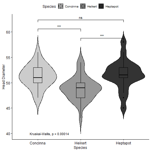
![caption](RmdWorkShop_files/figure-html/ggpubr violin-1.png)
]

.pull-right[

```r
ggviolin(df, 
         x = "Species",
         y = "`Head Diameter`",
         fill = "Species",
         palette = "grey",
         add = "boxplot", 
         dd.params = list(
           fill = "white")
         ) + 
  # Add significance levels
  stat_compare_means(
    comparisons = my_comparisons,
    label = "p.signif"
    ) + 
  # Add the global p-value 
  stat_compare_means(
    label.y = 40
    ) 
```
]
---

## ggpubr::ggerrorplot()

```r
ggerrorplot(df, x = "Species", y = "`Head Diameter`", 
            color = "Species", desc_stat = "mean_ci",
            palette= "grey",position = position_dodge(0.3), 
            size = 0.9)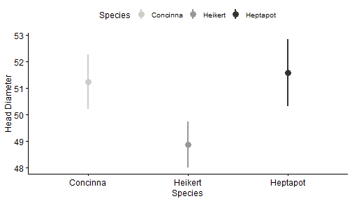
```

![caption](RmdWorkShop_files/figure-html/ggpubr error ci echo-1.png)
---

## GGally::ggpairs()

```r
ggpairs(df, columns = 2:4,
        lower = list(continuous = Mmisc::plot_trend_lines)) + 
  papaja::theme_apa()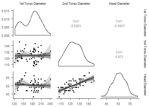
```

![Correlogram and Correlation Matrix.](RmdWorkShop_files/figure-html/ggpairs-1.png)

---

## knitr::include_graphics()
When plots are not generated from R code, we generate the images manually and pass their file paths to `include_graphics()` to include them in the output.

```r
knitr::include_graphics("figures/poweranalysis.png")
```

---

## Latex

We can use `$\LaTeX$` tricks!

Possible examples include:
```r
This sentence contains normal and $\textit{italic text}$.
```
This sentence contains normal and `$\textit{italic text}$`.

and also a bit more complex stuff:
```r
$$\begin{align} y|x &\sim Poisson(\lambda(x)) \end{align}$$
```
`$$\begin{align} y|x &\sim Poisson(\lambda(x)) \end{align}$$`

---

## Inline Text

```r
dt_print <- apa_print(dt , es = "pes")
```

We might want to reference some data in our text.
We _could_ type it.. (Note the use of `$\LaTeX$`)

```r
The effect of Instruction on response was not significant
 *F*(1, 38) = 0.31, $\mathit{MSE}$ = 506.86, *p* = .583,
 $\hat{\eta}^2_p = .008
```

prints out as:

The effect of Instruction on response was not significant `$F(1, 38) = 0.31$`, `$\mathit{MSE} = 506.86$`, `$p = .583$`, `$\hat{\eta}^2_p = .008$`

---

## Inline Text - Cont.

We can also automagically insert it:
```r
The effect of Instruction on response was not significant `r
dt_print$full_result$instruction`
```

prints out as:

The effect of Instruction on response was not significant `$F(1, 38) = 0.31$`, `$\mathit{MSE} = 506.86$`, `$p = .583$`, `$\hat{\eta}^2_p = .008$`

---

## Some output formats

.pull-left[
#### rmdformats::htmlclean
<img src="figures/rmdformats_htmlclean.jpg" width="1707" />

#### rmdformats::readthedown
<img src="figures/rmdformats_readthedown.jpg" width="1707" />
]

.pull-right[
#### rticles::plos
<img src="figures/plos.png" width="1555" />

#### rticles::PNAS
<img src="figures/PNAS.png" width="1495" />
]

---

## Knit

- Click the *Knit* button at the top of the RStudio scripts pane, OR:

```r
  rmarkdown::render("<file path>") 
```

---

## papaja Tables
### papaja::apa_print() and papaja::apa_table()

```r
dt_print <-
    apa_print(dt , es = "pes")

apa_table(dt_print$table)
```

A bit of cheating:

- This is a screenshoted Docx document
- We ran a Macro to fix font size and line spacing (we'll cover that later)

---

## papaja::apa_table() with caption and note

```r
apa_table(dt_print$table , 
          note = "this is a note",
          caption = "this is a caption")
```

Same cheats as before...

---

## Figure Captions and Cross-References
<img src="figures/papaja_cheat_plots.png" width="474" />

```r
In papaja we can also create cross-references, 
such as this. See Figure \@ref(fig:includegraphics).
```

---

## Citations

We can cite bibliography records from `Zotero` using the `citr` addin in rstudio.
<img src="figures/citr.png" width="468" />

---

## Papaja Workflow

Useful when the analysis takes more than a few seconds to run.

- Analysis as usual (R)
  - Get numbers (*M*s/*SD*s/etc), tables and figures to (at least almost) console-priniting shape
  - Save R environment to a file (e.g., "analysis.Rdata")
- Create new R Markdown file
  - Edit header
  - Load R environment from file (e.g., "analysis.Rdata")
  - Write Body (+ cite previous works)
  - Knit
  - Revise (IN R MARKDOWN, not output)
- Final adjustment on output (e.g. fix table font size with Word Macro)

---

## Fix tables with Word Macro
```VBA
Sub fixPapajaTables()
'
' fixPapajaTables Macro
'
'
    Dim tbl As Table
    For Each tbl In ActiveDocument.Tables
         tbl.Range.Font.Size = 10
         tbl.Range.ParagraphFormat.LineSpacing = 10

Next
    
End Sub
```

## Non-R Workflow

- Analysis as usual
  - Get numbers (*M*s/*SD*s/etc)
  - Save tables and figures as PNG/JPG graphic files
- Create new R Markdown file
  - ...
  - Write Body (insert numbers and graphics)
  - ...
- Final adjustment on output (probably not needed as the graphics were embedded as-is)

Remember non-R elements can be combined in an R workflow